Global predictions for the risk of establishment of Pierce’s disease of grapevines

Introduction

Pierce’s disease (PD) of grapevines is nowadays considered a potential major threat to winegrowers worldwide, causing huge economic losses that add up to more than 100$ milion in California alone. The causal agent of PD, the bacterium Xylella fastidiosa (Xf), is native to the Americas where it also causes vector-borne diseases on many economically important crops, such as citrus, almond, coffee and olive trees. In Europe, despite strict quarantine measures to protect the wine industry, PD has recently been established for the first time in vineyards on the island of Majorca, Spain. This finding, alongside the detection of PD in Taiwan, has raised concerns about its possible spread to continental Europe and other wine-producing regions worldwide.

A key trait of Xf’s invasive potential is its capacity of being transmitted non-specifically by xylem sap-feeding insects. Recently, the role of the meadow spittlebug, Philaenus spumarius, in the transmission of Xf in Europe has been confirmed. Furthermore, PD is a thermal-sensitive disease, with the temperature being a range-limiting factor. Several works have attempted to predict the potential geographic range of the Xf in Europe and worldwide using bioclimatic correlative species distribution models (SDMs). However, none of these works has explicitly included information on vectors’ distribution or disease dynamics. They hence provide little epidemiological insight into the underlying environmental causes underpinning or limiting a potential invasion. An alternative to overcome these limitations is to develop mechanistic models based on the physiology of the pathogen, coupled with epidemiological models that consider the disease dynamics while avoiding the difficulties of including transmission parameters for each of the PD potential vectors. In this work, we present a temperature-driven dynamic epidemiological model to infer where PD would have become endemic in different wine-growing regions worldwide from 1981 onward if we forced the introduction of Xf-infected plants. We show that transmission models based on the spatial distribution of the vector population (e.g. Philaenus spumarius in Europe) linked to temperature-driven frameworks accounting for Xf within host survival are key to develop accurate models for risk assesment.

The model

The effect of temperature on the symptom development process - A mechanistic model of Xf climatic suitability

We performed several inoculation assays to 36 grapevine varieties to elucidate the effect of temperature on the symptom development process. Basically, the plants where inoculated with the bacterium and the development of symptoms (as a binary outcome) was tracked in time. This experiments, together with previously measured data of Xf growth as a function of temperature, allowed us to develop a mechanistic framework capable to describe the symptom development process only from temperature data. The general idea is that, by knowing how fast bacteria grow at different temperatures, one can compute an approximation to the bacterial load of infected plants over a given time period if temperature data is available (Fig. 1a). Then, thanks to the inoculation assays, this approximated bacterial load (MGDD) can be translated into a probability of developing symptoms (Fig. 1c).

However, this is not the end of the story, as cold enough temperatures can then kill bacteria from infected plants! PD is very rarely found in zones in which the minimum average temperature of the coldest month (\(T_{min}\)) is below -1.1ºC, limiting its geographic expansion in the US. We then used this information to relate cold accumulation (CDD) to plant survival, or what is the same, to the probability of recovering from infection (Fig. 1b, Fig 1c). Finally, by combining symptom development and recovery, we developed a unified framework to model where PD can thrive or not given a particular weather. In essence, we just built a mechanistic model of climatic suitability for Xf within its grapevine hosts (Fig 1d).

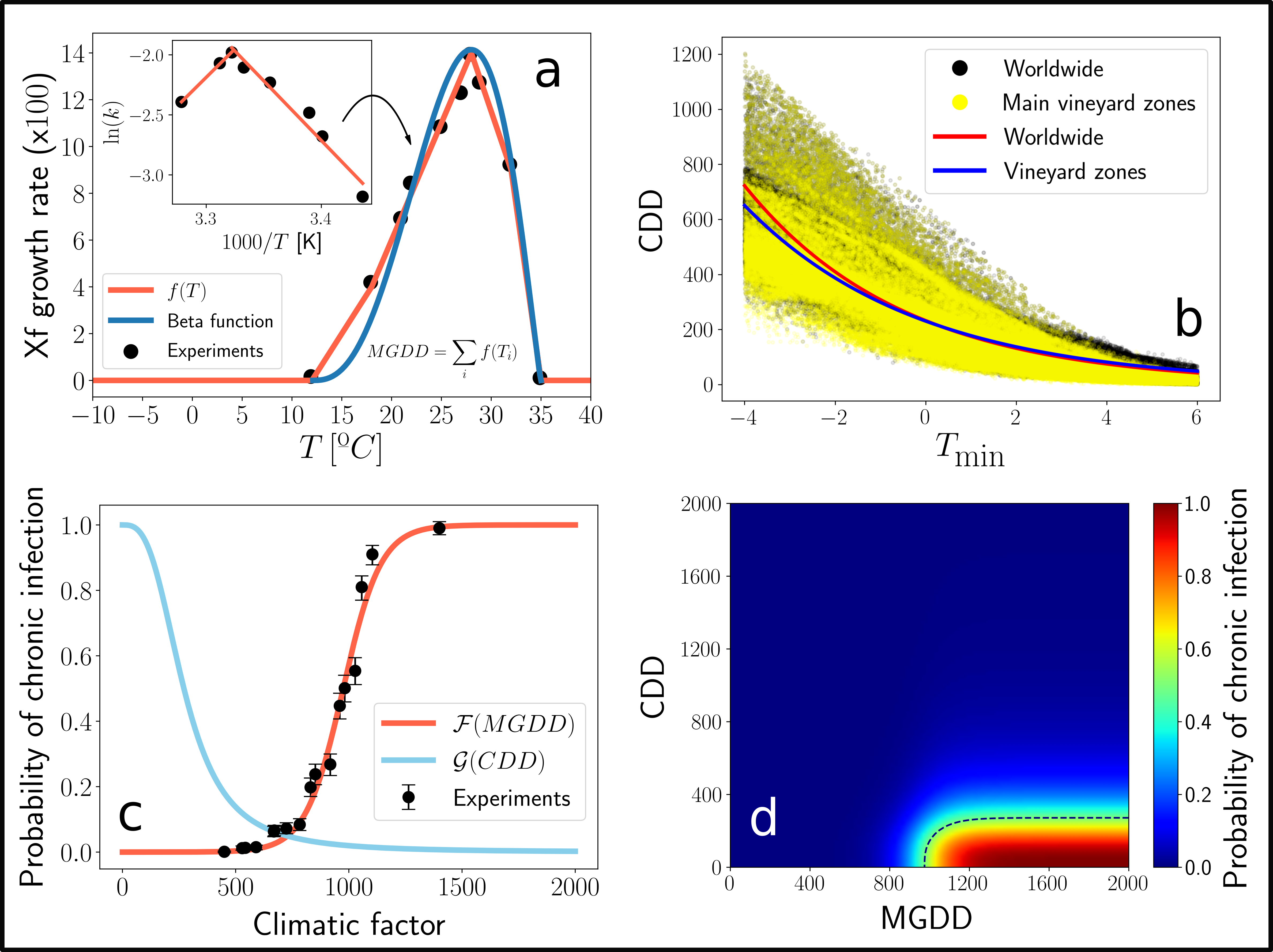
Fig. 1. Scheme of the mechanistic climatic suitability model.

The disease transmission model - Integrating the spatial distribution of the vector

Obviously, there will not be any risk of having the disease in a place where transmission from infected to susceptible plants cannot occur, even if the weather is perfectly suitable for the bacteria. To take this into account, we developed a compartmental model for vector-borne diseases suitable to describe Xf related diseases. This kind of models are customary used in mathematical studies of epidemic spreading (read this post for an introduction). The most important parameter of the model is the so-called Basic Reproductive Number, \(R_0\), which measures the average number of secondary infections produced by an initial infected plant in a fully susceptible population. In our case, the Basic Reproductive Number is given by

\[R_0 = \frac{\beta\alpha}{\gamma\mu}\frac{N_v}{N_H}\]

The important thing of the formula is that \(R_0\) depends linearly on $N_V$, the vector abundance. Thus, the more abundant the vector is in a given zone, the easier it will be for the disease to spread. This allows to include information of the spatial distribution and abundance of the vector in our model.

Fig. 2. Representation of the transmission model.

A temperature-driven dynamic epidemiological model for PD risk assesment

Finally, we had all the pieces to develop our complete model on PD risk. Information on the spatial distribution and abundance of the vector allow us to know how many new infected plants will an infected plant contribute to infect, while temperature data allow us to know how many of these new infections will indeed thrive. So only if this balance is positive, and mantained in time, an outbreak will occur. By joining the climatic suitability and transmission model in a single framework, we could develop our complete model for PD risk assessment. Indeed, the model can be summarised in a single simple equation for each location j under study

\[I_j(t)=\underbrace{I_j(t-1) \, e^{\gamma \, (R_0(j)-1)}}_\text{transmission layer} \overbrace{\Pi_j(t)}^\text{climatic layer} \ ,\]

from which we define the risk index as

\[r_j=\textrm{max}\left\{\frac{\log(I_j(\mathcal{T})/I_j(t_0))}{\gamma\, (R_0(j)-1)\, \mathcal{T}}, -1 \right\} \ .\]

The idea behind these equations is very simple. The first one computes the evolution of the infected population given a particular \(R_0\) (influenced by the vector abundance) and given a particular weather (\(\Pi(t)\)). The second one only standarizes the result of the former by dividing the infected population by its theoretical maximum (given by the epidemic process in optimal climatic conditions, \(\Pi(t)=1\)).

Fig. 3. Representation of the risk index.

Results

Once the model was developed, we proceeded to its calibration with spatiotemporal data on PD presence/absence in the US and Europe, which provided very nice results. Afterwads, it was ready to use! In Fig. 4 you can see the results of the model after its application in several wine-producing regions worldwide. For these locations, the information of the vector spatial distribution is missing, so that we used a fixed and homogeneous transmission scenario given by \(R_0=5\) (which was the value found for Europe).

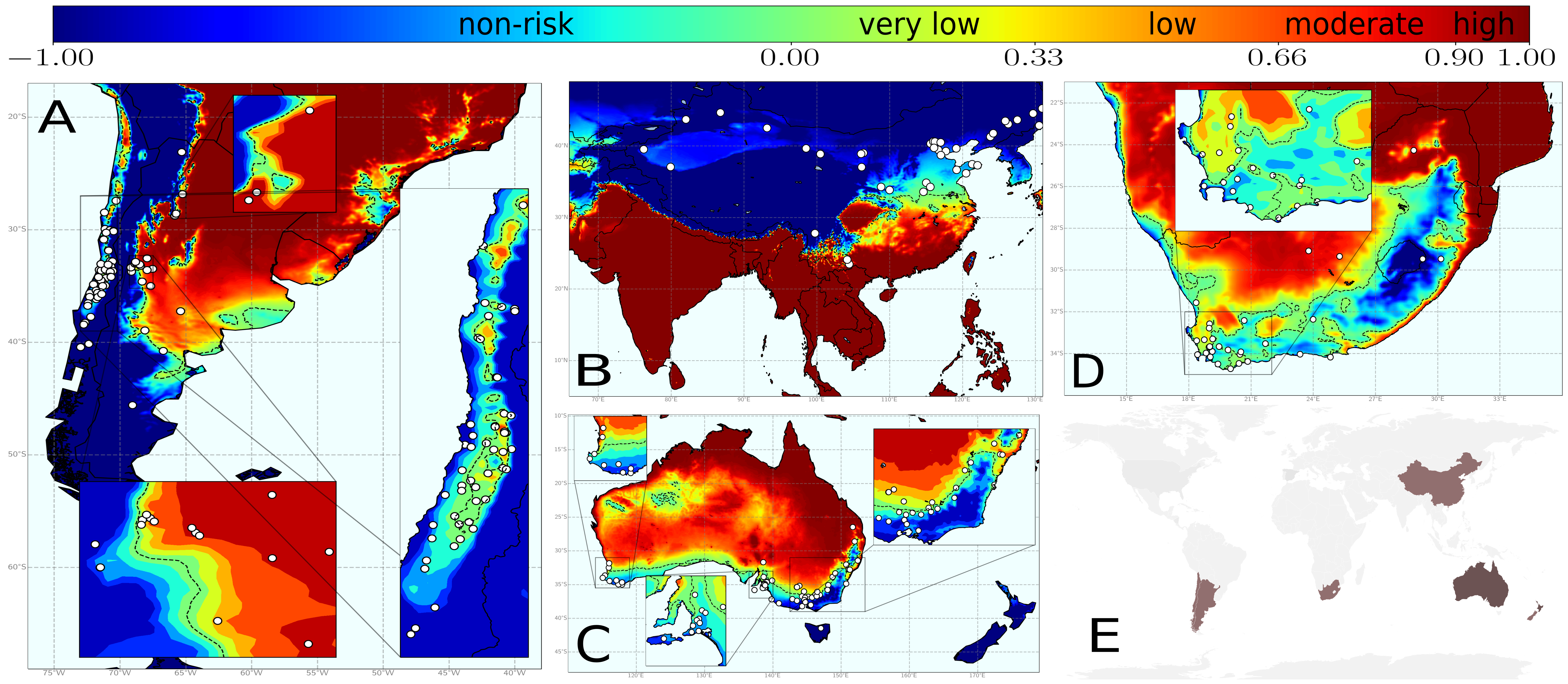
Fig. 4. Risk indices for different wine-growing regions worldwide using a fixed and homogeneous transmission scenario.

Nevertheless, information of the spatial distribution and abundance of the vector is indeed available for Europe. After incorporating it into the model (using different values of \(R_0\) for different locations) we found a drastic diminish of the risk, showing that there is no enough vectors in many climatic suitable regions for Xf to actually spread. Furthermore, the results accurately represented the currently affected zones as zones with high risk indices.

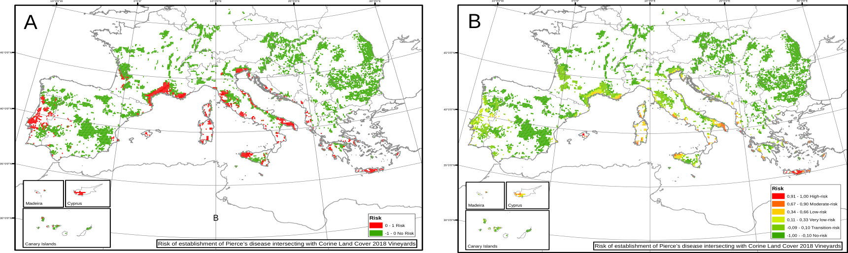
Fig. 5. Risk indices for European vineyards using a heterogeneous transmission scenario.

Conclusion

Our results are quite accurate, e.g. precisely representing the actual distribution of Xf-affected zones in Europe, but this is not for me the best part of our work. Perhaps as a physicist, I mostly like to admire the theoretical consistency and meaningfulness of some models, which I think is a strong point of ours. Although some other correlative models (e.g. AI) could perhaps equal the accuracy and predicting power of our mechanistic model, the fact that we can explain the fundamental factors that allow or not the expansion of PD is priceless.